Source Water Protection Project Methods

Parcels, or defined pieces of land, delineate how land is divided. Parcels are the key mapping unit for town operations including assessment, public safety, permitting and more.

Study Area

The study area for the project is all parcels that overlap drinking water watersheds (from the CT Dept. of Public Health) or aquifer protection areas (from the CT Dept. of Energy and Environmental Protection). This comes to 137,664 parcels from 121 of Connecticut's 169 towns, with a total area of 678,428 acres, covering approximately 19% of the state area. See the Viewer for a synoptic view.

Methods Overview

  1. Collect parcels
  2. Define metrics for surface water areas and metrics for ground water areas
    1. Collect input layers and summarize by parcel
    2. Apply scores for each sub-metric to each parcel, aggregate sub-metric scores to a single metric score
    3. Apply weight to each metric
  3. Calculate parcel rank, scale
  4. Apply bonus to parcels in both surface and ground water areas
  5. Exclude from ranking: parcels owned by a water company or the state, parcels too small or too developed
  6. Design, create, and share web tools

Methods

Parcels as base unit of measure

Connecticut parcels are currently maintained by individual towns. Until recently, there was no way to get each town’s parcel dataset without contacting them and making the request. Public Act 18-175 section 6[1], passed in 2018, requires towns to submit a digital parcel file to its COG each year. Now parcels can be downloaded from the State GIS Office at the Office of Policy and Management. There is not currently a standard for parcel drafting or for parcel attribution. Attributes contain non-spatial information about each parcel, such as map block lot, land use, ownership, etc. The lack of standardization makes it difficult to seamlessly combine town parcel datasets into a larger dataset.

Parcel GIS Work

The team started pilot work with parcels collected by state Councils of Governments (COGs) in 2021. The actual work commenced when the 2022 parcel data collect was complete and available for download.

Although the legislation made it easier to find and download parcels, there were still a lot of issues with data quality. Some examples of inconsistencies and needed to be remedied include:

  • some COGs provided their member towns parcels as separate town files, some as a single, merged file,
  • some parcel datasets overlapped, for example, the Department of Emergency Management (DEMIS) parcels covered their region 5, which overlapped with two COGs and many town datasets in the northwest part of the state,
  • condo complexes were treated differently in different datasets, like many tiny circles or squares, repeated parcels on top of each other many times (some over 300),
  • there were many cases of both parcel overlap and gaps at town boundaries,
  • some towns simply had messy GIS data, like overlapping duplicates that were difficult to find and sliver polygons,
  • some towns had polygons for rights-of-way (roads) and sometimes waterbodies that needed to be removed.


Each inconsistency had to be worked through before the parcels could be merged into a single dataset. After exploring the attributes, we decided that it was beyond the scope of this project to successfully merge them given different schema for each town and they were removed.

After merging all town parcel datasets, some new issues were evident including “null” polygons, “self intersections” and others that required removing polygons and/or repairing. Once a clean parcel file was ready to go, it was on to metrics.

Note: The CT GIS Office is working on improving parcel access and consistency. An single statewide parcel dataset with attributes will make this step far simpler and more accurate.

Metric identification

Metric Identification

The final list of metrics was determined using multiple sources. The biggest influence was the experience of the members of project team and advisors who know and understand the important characteristics that result in better water quality. The team also consulted outside experts and other similar projects.

We are aware of the dependent nature of these metrics and the ranking is just one way to combine them. We encourage anyone to use the individual metric layers or the tools to calculate and draw their own conclusions.

Metric calculations

The metric calculations methods can be grouped into two categories as follows.

Area and Percent

For metrics that use area and percent, the calculations are straightforward. Using GIS, we determined the area of overlap and the percent of the parcel area. For example, for the forest metric, we determined how much forest area overlapped with each parcel and what the percentage of the parcel.

Distance

A number of metrics require a distance calculation, for example, distance of a parcel from a waterbody or wetland. This may sound simple and it is when it is point to point. It is more complicated when the distance is between two polygons (a polygon is a shape with area) and distance can be calculated from the closest corner, the center, or somewhere else. To further add to the complication, the calculation needed to measure the distance from features within the watershed ONLY, even if a feature in another watershed was closer.

To illustrate, see the graphic below. The blue lines are basin boundaries. The small parcel, highlighted in cyan, is closer to the eastern waterbody (orange arrow) than the western waterbody (red arrow). In a standard GIS calculation, the distance to the eastern waterbody would be recorded as the shortest distance but this doesn’t make sense as it is part of a different watershed. The method used in the project calculates the distance from the parcel to the nearest waterbody in the SAME WATERSHED (the distance shown by the red arrow).

Distance calculation example

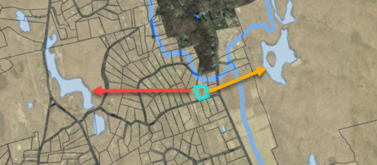
Example of distance calculation from a polygon to waterbody, where the red arrow is the correct distance because it is within the watershed, even though the orange area distance is shorter.

Metric classification and scoring

Each metric's values are divided into categories and each category is assigned a score ranging from 0 to 10. The more desirable the category, the higher the score.

For example, the sub-metric Distance to waterbody has four categories:

Category Score
0-15 feet (contains) 10 (most desirable)
15-300 feet 6.67
300-500 feet 3.33
>500 feet 0 (least desirable)

A parcel with a distance of less than 15 feet to a waterbody receives the top score of 10. It contributes the highest score possible to the rank. A parcel with a distance between 300 and 500 feet to a waterbody received a score of 3.33, meaning that this parcel contributed 1/3 as much as the top category.

Metric weighting

The metric weights determine how much influence an individual metric has on the final parcel rank. Metrics with higher weights are deemed more important by the project team. 

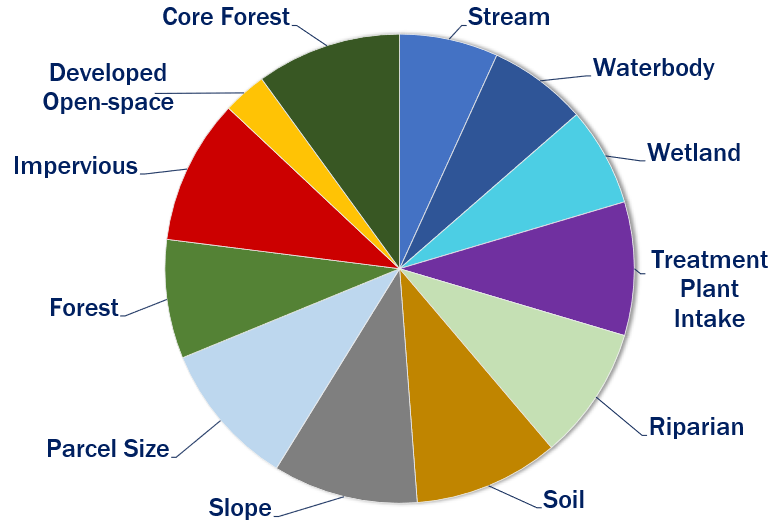
Surface Water Metric Weights

Metric Weight
Distance to streams 0.068
Distance to waterbodies 0.068
Distance to wetlands 0.092
Distance to treatment buffer intake 0.092
Contains stream bank/riparian 0.092
Soils 0.100
Slope 0.100
Parcel Size 0.100
Forest Cover 0.082
Impervious Surface 0.100
Developed Open Space 0.030
Core Forest 0.100
TOTAL 1.000

A pie chart helps visualize the metric weights shown in the table. The larger the slice of pie, the more contribution to the rank.

Pie chart view of surface water metric weights

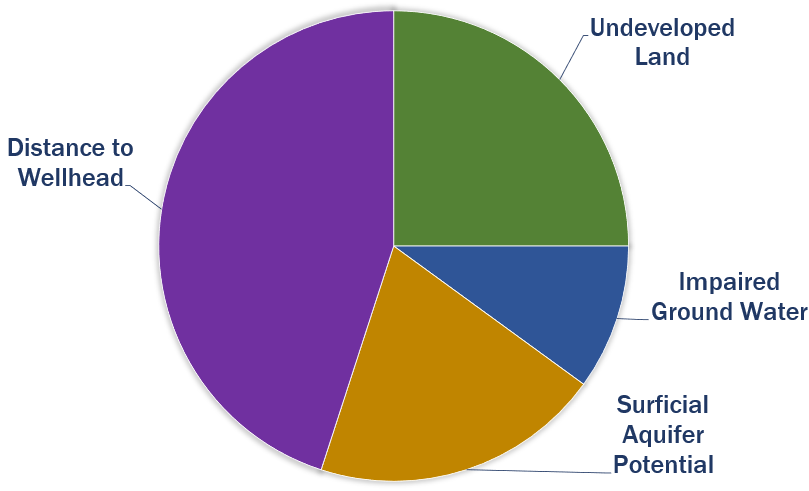
Ground Water Metric Weights

Metric Weight
Undeveloped land 0.250
Ground water quality 0.100
Surficial aquifer potential 0.200
Distance to wellhead buffer 0.450
TOTAL 1.000

A pie chart helps visualize the metric weights shown in the table. The larger the slice of pie, the more contribution to the rank.

Pie chart of ground water metrics

Sub-Metrics

Some metrics are made up of more than one metric, called a sub-metric. For example, the Distance to Waterbodies metric consists of BOTH (1) distance to waterbody and (2) percent of parcel that contains waterbody. Sub-metrics each contribute a piece to the full metric weight. In most cases when two sub-metrics are involved, the contribution is equal, or 50%. One exception is the Distance to Treatment Buffer metric where the sub-metric distance to intake buffer contributes 70% while the distance to intake reservoir contributes 30%. Another exception is the Slope metric where the area with extremely steep slope contributes 75% and the area of moderately steep slope contributes 25%.  The final exception is the Soils metric which is made of four sub-metrics, each of which contributes 25%.

Only one ground water metric, Undeveloped Land, consists of two sub-metrics and they are not divided equally. The area of parcel that is undeveloped contributes 70% and the percent of parcel that is undeveloped contributes 30%.

TIP! The sub-metric contribution values are included in the metric descriptions for both source water metrics and ground water metrics.

Example

As described above, the Distance to Treatment Buffer metric has a metric weight of 0.092 and includes two sub-metrics.

Sub-metric 1: distance to intake buffer, contributes 70% to metric weight.
Sub-metric 2: distance to intake reservoir, contributes 30% to metric weight.

Formula: Weight of sub-metric = metric weight x sub-metric contribution

Weight of Sub-metric 1 = 0.092 x 70% = 0.0644
Weight of Sub-metric 2 = 0.092 x 30% = 0.0276

Parcel Ranking

Parcel rank for a given parcel is calculated by summing the multiplication between a metric weight and its metric score for all the metrics.  See the Metric weighting section for more on how the contributing weights are determined.

Rank =   Weights x Metric Score

Since metric weights add to 1 and metric scores range from 0 to 10, parcel ranks range from 0 to 10. The higher the rank (close to 10), the more desirable the parcel.

Example

As described in the Metric weighting section, the Distance to Treatment Buffer metric has two sub-metrics: 1) sub-metric 1 (distance to intake buffer) with a weight of 0.0644, and 2) sub-metric 2 (distance to intake reservoir) with a weight of 0.0276. The categories and scores for these two sub-metrics are the same and shown in the table.

Category Score
0 - 15 feet 10
15 - 300 feet 6.67
300 - 500 feet 3.33
> 500 feet 0

An example parcel has a score of 10 for sub-metric 1 and a score of 6.67 for sub-metric 2. The rank of this parcel for the Distance to Treatment Buffer metric is calculated as

Rank of Sub-metric 1 = 0.0644 x 10 = 0.644
Rank of Sub-metric 2 = 0.0276 x 6.67 = 0.184

Rank contribution of the Distance to Treatment Buffer metric = 0.644 + 0.184 = 0.828

We repeat this calculation for all metrics and then sum up the rank contributions to derive the final rank for this parcel.

Scaled Rank

Because no parcel reached the total possible surface water rank of 10, the results were stretched, or scaled, to fill the full range of 0-10. This further separated parcel ranks making them easier to explore and better highlighted the most desirable parcels with high ranks. To be fully transparent, BOTH the actual rank and scaled rank are reported on the Parcel Information Panel (left side) of the Parcel Prioritization Viewer.

Stretched value example from dashboard

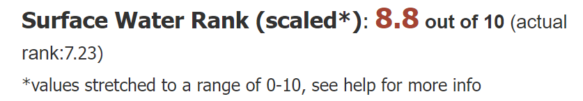
In this example, the ranking math resulted in a 7.23 out of 10. When the values were stretched so that the highest actual parcel rank is 10, this parcel receives a surface water rank of 8.8. The map layers and Parcel Priority Dashboard use the scaled rank throughout.

Exclusions and bonuses

Exclusions

Several characteristics disqualify the parcel from further consideration and therefore being part of the rank. The exclusions are:

  • parcels with an area less than 2 acres,
  • parcels that are more than 80% impervious surface,
  • parcels owned by a water company, and
  • parcels that are state-owned open space.

Bonuses

Bonus points were awarded to parcels that occur in both a drinking water watershed and an aquifer protection area. Bonus points are scaled based on the initial surface water and ground water ranks. Bonus points were not awarded for parcels that were excluded.

Surface Water Rank Ground Water Rank Bonus Awarded
>7 >8 2 points
5-7 6-8 1 point
3-5 3-6 0.5 point
0-3 0-3 0.25 point

Significant Environmental Hazard Locations

Environmental hazards are important because it is not a useful preservation area if the parcel is already contaminated. The Significant Environmental Hazard Locations layer is provided by CT DEEP and provides the status of hazardous conditions, including open, controlled, and resolved conditions. The points are included in the Parcel Prioritization Viewer and parcels that contain a hazard point of any kind are flagged in the Parcel Information panel with text ** Identified as Significant Environmental Hazard Site. The presence of a site should not immediately exclude the parcel from consideration, but does warrant further investigation. 

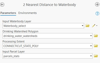
Repeatability through GIS tools

We recognize that this analysis is a point in time. Data layers will improve, including the base parcels, and the analysis will need an update. Each step of the analysis was created as a tool within a toolbox in ArcGIS Pro. The tools are grouped based on the metric. The tools also allow for data and data layer updates and enable the methods to be applied to other regions that may have different input datasets.

Sample of GIS toolbox  Sample tool interface

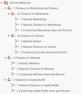
If you are interested in the tools, please contact us at clear@uconn.edu and mention the Source Water project GIS toolbox.

Sharing the results

The results of the analysis are available in two interactive tools.

The Parcel Prioritization Viewer is map-centric. It includes all of the metric calculations as well as map layers for the metric inputs and metric results. Visit the Parcel Prioritization Viewer Help for detailed instructions and capabilities of the viewer.

The Parcel Priority Dashboard focuses on finding parcels based on their rank or other criteria. Visit the Parcel Priority Dashboard help for detailed instructions and capabilities of the dashboard.

Metrics

There was extensive discussion regarding each metric used in the project. In some cases, experts joined the discussion and informed the decisions. One set of metrics was used for parcels in a drinking water watershed (surface water) and an entirely different set of metrics was used for parcels in an aquifer protection area (ground water).

Surface Water Metrics

Distance to streams

Streams can carry pollutants and quickly degrade water supplies. A parcel either close to or containing streams is important for surface water quality.

Inputs: National Hydrography Dataset (NHD) streams and rivers

Sub-metrics each contribute equally.

  1. Distance to streams (feet) within the corresponding drinking water watershed
  2. Length of streams within a parcel (feet)

Distance to waterbodies

Waterbodies can store and release pollutants and impact water quality. A parcel either close to or containing a waterbody is important for surface water quality.

Inputs: National Hydrography Dataset (NHD) pond/lakes and reservoirs

Sub-metrics each contribute equally.

  1. Distance to waterbody (feet) within the corresponding drinking water watershed
  2. Percent of parcel containing waterbody

Distance to wetlands

Wetlands are important for water quality as the filter pollutants. Parcels containing wetlands are valuable for water quality.

Inputs: Hydric Soils from the Natural Resources Conservation Service (NRCS)

Sub-metrics each contribute equally.

  1. Distance to wetlands (feet) within the corresponding drinking water watershed
  2. Percent of parcel containing wetlands

Distance to treatment intake buffer

When water is closer to a treatment plant intake or intake reservoir, it has fewer opportunities to be naturally cleaned and therefore potentially greater impact to water quality.

Inputs: A buffer area containing the intake.

Sub-metrics contribute differently for this metric. The distance to treatment plant intake zone has a higher weight (0.7) than the second metric, distance to intake reservoir (0.3). Both are important, but the intake area is critical.

  1. Distance to treatment plant intake zone (feet)
  2. Distance to intake reservoir (feet)

Contains stream bank/riparian

Parcels with more area in the riparian zone are important for water quality. Activities and land cover within the riparian zone can have a greater impact on the water resources than those outside of the riparian zone. The team evaluated and assessed different sizes and decided on a 50 meter (164 feet) buffer from the waterbody edge or stream line. This metric compares the buffer zone area with the parcel.

Inputs: National Hydrography Dataset (NHD) pond/lakes and reservoirs

Sub-metrics contribute equally.

  1. Area of parcel that that contains riparian zone (acres)
  2. Percent of parcel that contains riparian zone

Soils

The soils metrics and options were particularly complicated and confusing. The team met with the state soil scientist and other water experts multiple times and decided on four sub-metrics, listed below.

Inputs are from the USDA NRCS Soil Data Viewer which does the calculation for each desired metric with user-defined settings. The output is a table with value(s) for each soil polygon. The four selected soil metrics are as follows:

  • K Factor (under Soil Erosion Factors), Whole Soil over Rock Free after consultation with the state soil scientist.

Erosion factor K indicates the susceptibility of a soil to sheet and rill erosion by water. The estimates are based primarily on percentage of silt, sand, and organic matter and on soil structure and saturated hydraulic conductivity (Ksat). Values of K range from 0.02 to 0.69. Other factors being equal, the higher the value, the more susceptible the soil is to sheet and rill erosion by water.

  • Depth to Water Table

"Water table" refers to a saturated zone in the soil. It occurs during specified months. Estimates of the upper limit are based mainly on observations of the water table at selected sites and on evidence of a saturated zone, namely grayish colors (redoximorphic features) in the soil.

  • Depth to Any Soil Restrictive Layer (depth to restriction)

A "restrictive layer" is a nearly continuous layer that has one or more physical, chemical, or thermal properties that significantly impede the movement of water and air through the soil or that restrict roots or otherwise provide an unfavorable root environment. Examples are bedrock, cemented layers, dense layers, and frozen layers. This theme presents the depth to any type of restrictive layer that is described for each map unit. If no restrictive layer is described in a map unit, it is represented by the "greater than 200" depth class. 

  • Saturated Hydraulic Conductivity (Ksat), standard classes

Saturated hydraulic conductivity (Ksat) refers to the ease with which pores in a saturated soil transmit water. The estimates are expressed in terms of micrometers per second. They are based on soil characteristics observed in the field, particularly structure, porosity, and texture. The numeric Ksat values have been grouped according to standard Ksat class limits. 

Because a parcel can intersect multiple soil polygons, the values for intersecting soil polygons needed to be aggregated to represent a parcel. For each soil metric, a given parcel was summarized as an area-weighted average value by multiplying values of intersecting soil polygons with their corresponding percent areas of the parcel.

Sub-metrics contribute equally. Four sub-metrics make up the soil metric. After many discussions, the team felt that these four metrics capture the important features of soil for the purpose of surface water quality protection.

  • Percent of parcels with k factor > 0.4 (highly erodible) 
  • Percent of parcel with soil depth to water table less than 50 cm
  • Percent of soils with a depth to restrictions < 60 inches
  • Percent of soils with a Ksat > 1 (high conductivity)

Slope

Steep slopes have faster run-off and erosion potential, and less time for water absorption.

Inputs: 2016 statewide, 1 meter Lidar digital elevation model (DEM) which is a raster layer of bare earth elevation. A slope percentage function was applied to the 2016 DEM to calculate slope. An ArcGIS toolset was then developed to compute the percent area of extremely steep slope (i.e. >15%) and moderately steep slope (i.e. 8-15%) for each parcel.

Sub-metrics are weighted differently. The percent of parcel with extremely steep slope sub-metric is weighted heavier (0.75) than the percent of parcel with moderately steep slope (0.25) sub-metric.

  1. Percent of parcel with extremely steep slopes (> 15%)
  2. Percent of parcel with moderately steep slope (8-15%)

Parcel size

Larger parcels result in a greater area of land that is persevered. It is also easier to protect fewer, large parcels than many small ones.

Inputs: Parcel layer used in this study.

Sub-metric

  1. Parcel area (acres)


Note that parcel less than 2 acres in size are excluded from ranking. See the Exclusions and bonuses help section.

Forest cover

Forest cover provides valuable benefits for water quality.

Inputs: 2016 CT high resolution land cover, forest classes (deciduous forest, evergreen forest, mixed forest, forested wetland)

Sub-metric

  1. Percent of parcel that is forest

Impervious area

Runoff from impervious surface prohibits infiltration and adds pollutants to waterways.

Inputs: 2016 Connecticut high resolution C-CAP land cover, impervious classes (high intensity developed, medium intensity developed, low intensity developed)

Sub-metric

  1. Percent of parcel that is impervious cover

Turf and grass

Development and maintenance of constructed materials and managed grasses contributes pollutants and degrades water quality.

The developed open space class of the statewide, high resolution land cover was used for this metric. Developed open space is defined as:

areas with a mixture of some constructed materials, but mostly managed grasses or low-lying vegetation planted in developed areas for recreation, erosion control, or aesthetic purposes. These areas are maintained by human activity such as fertilization and irrigation, are distinguished by enhanced biomass productivity, and can be recognized through vegetative indices based on spectral characteristics. Constructed surfaces account for less than 20 percent of total land cover.

Inputs: 2016 CT high resolution land cover, developed open space class

Sub-metric

  1. Percent of parcel that is developed open space

Core forest

Core Forest was added by recommendation from the Advisory Committee. Core forest is determined from the forest fragmentation data layer produced by UConn CLEAR. The layer was created by applying a model that classifies each forest pixel into a forest fragmentation category – patch, edge, perforated, and core (small (<250 acres), medium (250-500 acres), large (>500 acres)). The core forest areas are desirable in this study as they indicate patches of forest that are some distance from non-forest and provide great value to water quality.

Inputs: CLEAR’s 2015 Connecticut Changing Landscape 30 meter land cover forest fragmentation layer

Sub-metrics

  1. Area that is core forest (acres)
  2. Percent of parcel that contains core forest

Agricultural land

Agricultural area was calculated for parcels but not included in the ranking.

Inputs: 2016 CT high resolution land cover, agricultural classes (cultivated crops, pasture/hay)

Sub-metric

  1. Area that is agriculture (acres)
  2. Percent of parcel that is agriculture
Ground Water Metrics

Undeveloped land

The more undeveloped land, the higher the value for ground water quality due to infiltration and lack of pollutants. The team considered different options for this metric including forest land cover, core forest, and the State Plan of Conservation and Development, and ultimately decided on undeveloped classes from the land cover.

Inputs: CT 2016 high resolution land cover undeveloped classes (all classes except impervious and developed open space)

Sub-metrics contribute differently for this metric. The area of parcel that contains undeveloped land sub-metric has a higher weight (0.7) than the second metric, percent of parcel that contains undeveloped land (0.3).

  1. Area of parcel that contains undeveloped land (acres)
  2. Percent of parcel that contains undeveloped land

Ground water quality

It’s not a useful preservation area if the groundwater is already contaminated. The metric is a presence or absence of impaired groundwater.

Inputs: Ground water quality layer from CT DEEP. Impaired groundwater classes are GB, GC, GA-impaired, and GAA-impaired. Other classes (GA, GAA) are not impaired.

Sub-metrics

  1. Presence of impaired groundwater

Surficial aquifer potential

Areas with high surficial aquifer potential and more valuable for protection due to their ability to store and transmit water.

Inputs: Surficial Aquifer Potential layer from CT DEEP.

High surficial aquifer potential is identified by areas with coarse deposits with depths greater than 50ft on the DEEP Surficial Aquifer Potential dataset. The explanation on the CT DEEP Surficial Aquifer Protection Map was very helpful in determining the metric classes.

The thicker and coarser-grained deposits have higher potential for water supply development. The most productive surficial aquifers in Connecticut are sand and gravel deposits originating from glacial meltwaters. These deposits are mapped where they occur at the surface and where they occur beneath fine grained deposits.

Coarse-grained glacial deposits have the greatest potential to both store and transmit water. The locations and thickness of these aquifers are of utmost importance for water management. Coarse-grained deposits of thicknesses greater than 50’ are considered to have the greatest long term potential ground water yields, particularly where they occur near large rivers and streams. Where coarse-grained deposits have a water saturated thickness of 10’ or greater, moderate to very large ground water yields of 50-2000 gallons per minute have been documented. The saturated thickness of these deposits has not been mapped statewide. Therefore, the overall thickness of these deposits may be used as a proxy for saturated thickness in that, given equal recharge, a greater coarse grained deposit thickness would have a higher potential of containing a greater volume of saturated material.

Sub-metrics

  1. Percent of parcel that contains coarse deposit depths greater than 50 ft

Distance to Wellhead

The closer the parcel is to a wellhead buffer, the more valuable for protection.

Inputs: Wellhead buffer zones as provided by the Department of Public Health.

The metric calculates the shortest distance between a parcel and its nearest wellhead buffer.

Sub-metric

  1. Distance (feet) to wellhead buffer

Support for this project was provided by the Connecticut Council on Soil and Water Conservation, in partnership with the Connecticut Department of Public Health.

CT Council on Soil and Water Conservation logo    Department of Public Health logo